Want to help out or contribute?

If you find any typos, errors, or places where the text may be improved, please let us know by providing feedback either in the feedback survey (given during class) or by using GitHub.

On GitHub open an issue or submit a pull request by clicking the " Edit this page" link at the side of this page.

3 Pre-course tasks

In order to participate in this course, you must complete everything in this pre-course tasks section and finish with completing the survey at the end. These tasks are designed to make it easier for everyone to start the course with everything set up. For some of the tasks, you might not understand why you need to do them, but you will likely understand why once the course begins.

Depending on your skills and knowledge, these tasks could take between 3-5 hrs to finish, so we suggest planning a full day to complete them. Depending on your institution and how they handle installing software on work computers, you also might have to contact IT very early to make sure everything is properly installed and setup.

3.1 Tasks to complete

Here’s the list of tasks you need to do. Specific details about them are found as you work through the tasks.

Read the Learning objectives in Section 3.2 for the pre-course tasks (below).
Read the “How to read the website” (on a new website).
Follow the installation instructions (on a new website). Install a version of R, RStudio, and Git that is as updated as possible. For some people, depending on their institution, this task can take the longest amount of time because you have to contact your IT to install these packages.
Read about R in Section 3.4.
Read about and become familiar with RStudio in Section 3.5.
Install necessary R packages in Section 3.6.
Read some of the course sections on Git, configure Git on your computer, and create a GitHub account in Section 3.7.
Run the code in these sections that checks to see if everything works (you’ll later need to paste this output into the survey).
Read about the basic course details in Section 3.8.
Read the Code of Conduct.
Complete the pre-course survey. This survey is pretty quick, maybe ~10 minutes. There will be some bits from the tasks that you will need to paste into this survey.

Check each section for exact details on completing these tasks.

3.2 Learning objective

In general, these pre-course tasks are meant to help prepare you for the course and make sure everything is setup properly so the first session runs smoothly. However, some of these tasks are meant for learning as well as for general setup, so we have defined the following learning objectives for this page:

Describe what R is, how it fits within a research environment, and why researchers increasingly use it.
Navigate some of the basic uses and features of RStudio, as well as understand the difference between R and RStudio.
Explain the differences between R code, R functions, R scripts, and R packages, and how we will use each of them.
Become aware of the tidyverse set of packages, which we will be teaching mostly in this course.
Become aware of what version control is and what Git is.

3.3 Programs to install

Make sure to install as updated versions of R, RStudio, and Git as possible by following these installation instructions on the Guides website. For some people, depending on their institution and their specific computer, this task can take the longest amount of time because you have to contact your IT to install these packages or do troubleshooting because of issues specific to your computer setup. It is extremely difficult to predict who will and who won’t have issues with these installation tasks.

3.4 What is R?

During this course, we will be spending most of our time in RStudio. RStudio is an “environment” that we use to interact with R. R is like an engine, while RStudio is like the tools we use to actually work with that engine. Prior to taking a look at what RStudio looks like, let’s talk briefly about R as a programming language.

R is a free programming language/environment used in statistical computing, data analytics, and scientific research. R is used to clean, organize, analyze, and report on data. R has powerful visualization features, so it is a particularly useful tool for creating charts and figures. R is different from SPSS and other statistical programs in that you run analyses by typing commands in a console rather than using click-based, drop-down menus.

In recent years, R has become one of the most popular languages among statisticians and data scientists for several reasons:

It is open source, so you are able to see how exactly a, for instance, statistical method works.
It runs on all platforms (Windows, macOS, Linux).
It is highly compatible with other programming languages.
It provides access to a vast amount of packages that can complete nearly any task or statistical approach.
There is a huge online community to help you problem-solve any issue.
It is free, which means you can continue using the skills you gain in R throughout your entire career without worrying about expensive licensing fees (for example, if your employer can’t or doesn’t pay for the software).

However, like many programming languages, R is not easy to learn. Some functions are spread across packages, which means that you need to have prior knowledge of packages in order to implement some commands. R can also be slower than other programming languages. Nonetheless, R offers such a supportive community and rich functionality that it is worth the challenge!

3.5 Getting familiar with RStudio

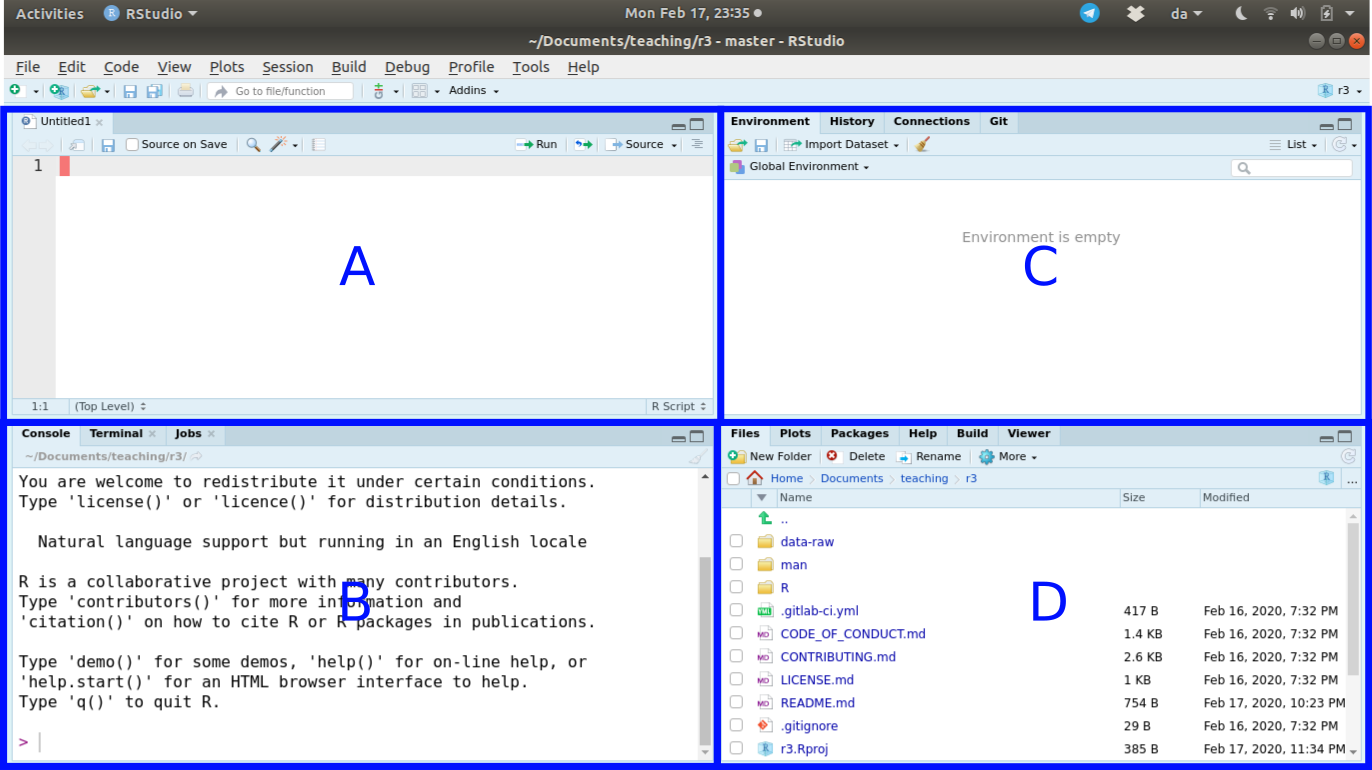
Let’s start learning about RStudio and how to use it. Check out Figure 3.1 below. You can see that RStudio has four “panels”, dividing the screen into the four sections.

Note: This image, along with the other images and videos below, may look slightly different from your own computer depending on your operating system and other settings.

While you can customize where the individual panels go, the default layout is how the panels are shown.

Panel “A” is the panel that shows the “scripts”, which we will be using a lot during the course. You may or may not see this panel when you open RStudio for the first time. This panel is where you write R code that will be saved as a file.
Panel “B” is the Console. This is where R commands are sent and evaluated by R. This is the “engine”. No R code written here is saved. Almost all of the tasks in this course will be entered through the Console.
Panel “C” contains the Environment, History, Connections, and Git tabs. In this course, we will only be using the Environment and Git tab.
Panel “D” has the Files, Plots, Packages, Help, Build, and Viewer tabs. For this course, we will only be going over the Files, Plots, Packages, and Help tabs. There can be slight differences in your layout of tabs in each panel.

While we will spend part of the course using an R script to play around with code, we will also be learning and using R Markdown / Quarto (.Rmd or .qmd files). R Markdown / Quarto is a dynamic and invaluable tool that will help make your analysis more reproducible. Quarto is an upgraded version of R Markdown but can also use R Markdown. Throughout the rest of the course, we will write and talk about Quarto, but we mean both Quarto and R Markdown. We will explain this in more detail in Chapter 8.

Quarto allows you to interweave chunks of code along with text and images. R runs the code and inserts the code output into the Quarto file. The Quarto document can be converted into a wide range of document types, including MS Word, PDF, or HTML. Some researchers write and manage entire papers, theses, websites, or books using Quarto, as it can make things easier to organize and maintain. In fact, this website is written with Quarto.

3.6 Installing R packages

Now that you have RStudio and R on your computer, we need to install the R packages we’ll use in the course. R packages are bundles of R code that other people have written. There are so many R packages available that there is likely an R package for anything you’d like to do in R. Making use of R packages can greatly help you out when doing your research.

Before we continue, we need to briefly explain what some terms mean.

R code is any individual piece of text that R interprets as commands to do something. For instance, mean() is a complete piece of text that tells R to calculate the mean of some numbers.
- R code is essentially split into two types: objects (like a dataset) or actions (called functions). For the most part, whenever you see code with () at the end (at least in this course), that means it is a function.
- A function is a set of bundled R code that performs a specific task. Like the example mean() above.
R script is any file with the ending .R that contains R code that completes tasks in a sequence (from the top of the file to the bottom).
R package is a set of R scripts that contain multiple bundles of R code (mostly these bundles are functions, but can sometimes be data) that work together to expand on or improve R code and R functionality.

For this course, we will be focusing on R packages that are powerful and general-purpose enough to help you in multiple aspects of your research. To install these packages, we’ll need to install the r3 helper package. For that, we’ll need to first install the pak package. Watch the video (no audio) below to see how to do this:

Or paste the following code into the RStudio R Console:

install.packages("pak")

Copy and paste the function below into the RStudio Console. Hit Enter and the r3 helper package will be installed. Watch the video below to see how to do this. Note, what you see in the video (no audio) may look different from yours.

pak::pkg_install("rostools/r3", upgrade = TRUE)

You might encounter an error when running this code. That’s ok, if you restart R by going to Sessions -> Restart R and re-running this code, it should work. If it still doesn’t, try to complete the other tasks, complete the survey, and let us know you have a problem in the survey.

It is important to understand what you are doing when you enter a function like something::something(). In the example of pak::pkg_install(), you would “read” this as:

R, can you please use the pkg_install function from the pak package?

You could load the package with library(pak) and then run the pkg_install() function. However, using the :: (pronounced “colon colon”) tells R that we want to use a function directly from a package. We prefer this way as we only want to use the pkg_install() function from the pak package without having to load all the other functions. We will be using :: often during this course.

Most of the packages we will be using in this course are bundled together into one package called tidyverse. This package is a collection of packages that are designed for common tasks in data science, ranging from data exploration to data visualization. As the name suggests, tidyverse is an attempt to organize the “universe” of data analysis by providing packages that guide workflows and lead to more reproducible analysis projects. To install all the packages we will use for this course, copy and paste this command into the R Console:

r3::install_packages_introduction()

Like with the installing of r3 in the video above, this will take some time to install everything. Normally, to install packages, you would type this in the Console (you don’t need to do this):

install.packages("tidyverse")

The specific packages from tidyverse that we will use are ggplot2 and dplyr. These packages provide a set of tools for the most common data analysis tasks and have excellent documentation and tutorials on how to use them.

dplyr (along with a complementary package tidyr) is a package that is very popular and contains important data manipulation functions, including functions that select and/or create variables depending on certain conditions. dplyr is built to work directly with data frames (rectangular data like those found in spreadsheets), and has an additional feature to interact directly with data stored in an external database such as in SQL. Working with databases is a powerful way to work with massive datasets (100s of GB), more than what your computer could normally handle. Working with massive data won’t be covered in this course, but see this resource from Data Carpentry to learn more.
ggplot2 is a data visualization package that can be used to create bar charts, pie charts, histograms, scatterplots, error charts, and more. It uses a “grammar” as a way to construct and customize your graphs in a layered, descriptive approach.

3.7 Setting up Git and GitHub

We’ll cover more about Git and GitHub during the course, but for now, please read Section 6.1, Section 6.2, and Section 6.3. During the course you will read them again and we will verbally explain it in more detail. Why repeat this twice? Because Git and version control are some of the more difficult things you will learn in this course and because they are fundamentally very different ways of working in your computer than you are probably used to. They require changing how you see and interact with your projects and computer in pretty big ways. So we want you to read this now so you can start to mentally process the concepts we will cover. Then we’ll get you to read it again during the course, to reinforce the concepts.

After reading about Git, we need you to prepare things so that you are ready for the course. In order to use Git properly, you need to inform your computer that you are using Git. The r3 course helper package has a function to help with this. Type in the RStudio Console:

r3::setup_git_config()

Hit enter and follow the instructions. Finally, type and run this next function to make sure everything is working with your setup. When you complete the survey later, you will need to copy and paste the output of this function.

r3::check_setup()

After you are done, you need to create a GitHub account. Make note of your username, as we will ask you for it in the pre-course survey. Make sure to remember your password, either write it down somewhere or (even better) use a password manager to store your password for you.

Note: GitHub is a company and website, while Git is a software. There is sometimes confusion about these two things since they both say “Git”. It’s important to distinguish that they are two separate things.

3.8 Basic course details

Most of the description of the course is found in the syllabus (Chapter 1). While you may have signed up to this course to learn more about R, you should know that conducting reproducible research goes beyond R and RStudio. As such, we will be spending a lot of time exploring other tools that are used in conjunction with R, to improve the structure and transparency of your work. This course is designed to not only introduce you to R, but also to show ways of conducting reproducible research and data analysis in R.

If you haven’t read the syllabus, please read it now. Read over what the course will cover, what we expect you to learn by the end of it, and what our basic assumptions are about who you are and what you already know. At the end of this section, we’ll ask you a few questions to see if you understand what you’ll learn in the course.

One goal of the course is to teach about open science, and true to our mission, we practice what we preach. The course material is publicly accessible (all on this website) and openly licensed so you can (re-)use it for free! The material is organized in the order that we will cover it in the course.

While the course will include lots of hands-on work during the sessions, the final group project assignment (Appendix B) will allow you to practice everything you’ve learned in a team setting. Please read it to get familiar with what is expected of you.

We have a Code of Conduct. If you haven’t read it, read it now. The survey involves a question about Conduct. We want to make sure this course is a supportive and safe environment for learning, so this Code of Conduct is quite important.

You’re almost done. Please fill out the pre-course survey to finish this section, either at this link.

See you at the course!